
Introduction
Data and Machine Learning
When it comes to talking about Machine Learning, it’s clear that it is the science (and art) of programming computers that learn from data [1]. However, this definition raises some questions, and the first one is: data? Excel spreadsheets?
The first thing people think (or at least that’s the first thing I thought) is structured data, such as .xlsx or .csv files. However, everybody says that "there is data everywhere," and one of my favourites is images (at the end of the day, images are just an array of numbers).
The tasks made by a computer on digital images or videos are under the field of Computer Vision. When Computer Vision is combined with Deep Learning (a Machine Learning area focused on Artificial Neural Networks), exciting projects and applications arise.
There are many Computer Vision tasks where Deep Learning has been involved (such as image classification and object detection) thanks to the implementation of Convolutional Neural Networks (CNN).
Classical Machine Learning instead of Convolutional Neural Networks
It is clear that in the face of any image classification problem, CNNs are the most suitable; however, in this project, I wanted to find a solution through the classical Machine Learning algorithms.
Maybe some readers are wondering why I’m doing this. The short answer is that I wanted to experiment with Feature Extraction methods and explore the limits of classical Machine Learning algorithms.
Disclaimer
In this project, I aim to explore how to solve this problem. The methodology is stipulated in Facial Expression Classification Based on SVM, KNN and MLP Classifiers by Hivi Ismat Dino and Maiwan Bahjat Abdulrazzaq.
Data and The Curse of Dimensionality
You can download the images and CSV files here
At small scales, physics phenomena behave differently from the ordinary scale (Quantum Physics vs Classical Physics); similar behaviours happen at higher dimensions.
A two-dimensional vector has two components and lives in a two-dimensional space:
a three-dimensional vector has three components and lives in a three-dimensional space:
and so on:
Intriguing things happen in high-dimensional spaces, for example:
- Most points in a high-dimensional hypercube are very close to the border [1]
- The average distance between two points in a hypercube is significant. For example, in a three-dimensional cube, the average distance between two random points is 0.66; but in a 1,000,000-dimensional hypercube, the average distance between two points is 408.25 [1].
What’s happening? Why does it happen? Well, there’s plenty of space in high dimensions. As a result, the data is very sparse, causing new instances to be far away from the training data, making the prediction less reliable than datasets with lower dimensions [1]
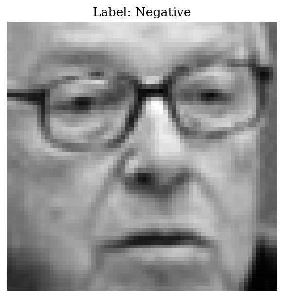
The dataset used is a collection of face images expressing one of two emotions: positive or negative. The images are 64×64 pixels, and if each image is transformed into a hyper-vector, we end up with a 4096 feature dataset, and that’s a lot of dimensions.
How could it be solved?
For this case, there are many ways of dealing with it, but the ones to explore are:
- Feature Detection.
- Dimensionality Reduction.
Feature Detector: Histograms of Oriented Gradients (HOG)
Histograms of Oriented Gradients (HOG) is a feature descriptor proposed by Dalal et al. in 2005 [2]. This descriptor computes the change of pixel luminance around a specific pixel. This change is given by a gradient (vector of change) with a magnitude m and angle 𝛉 (Eq. 1 and Eq. 2):
If you want to go deeper into this technique, I recommend the following video (here).
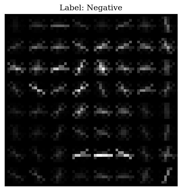
By applying this technique, the number of features changed from 4096 to 1764 (a reduction of 60%).
HOG can be found on the library scikit-image
from skimage.feature import hog
Dimensionality Reduction: Principal Component Analysis
Thanks to HOG, the dimensions went down but not enough; a next step had to be made.
Principal Component Analysis (PCA) is one of the most popular methods to reduce the number of features in a dataset. This unsupervised learning algorithm finds the linear projection that preserves the maximum amount of information. In other words, PCA finds the hyper-plane that maximizes the dataset variance [1].
Like K-Means, we have to declare the number of clusters we want; with PCA, we must give the number of features we want to reduce the dataset. The standard criteria used to find the optimal number of features is when the explained variance is not significantly increasing, similar to the Elbow Method on K-Means.
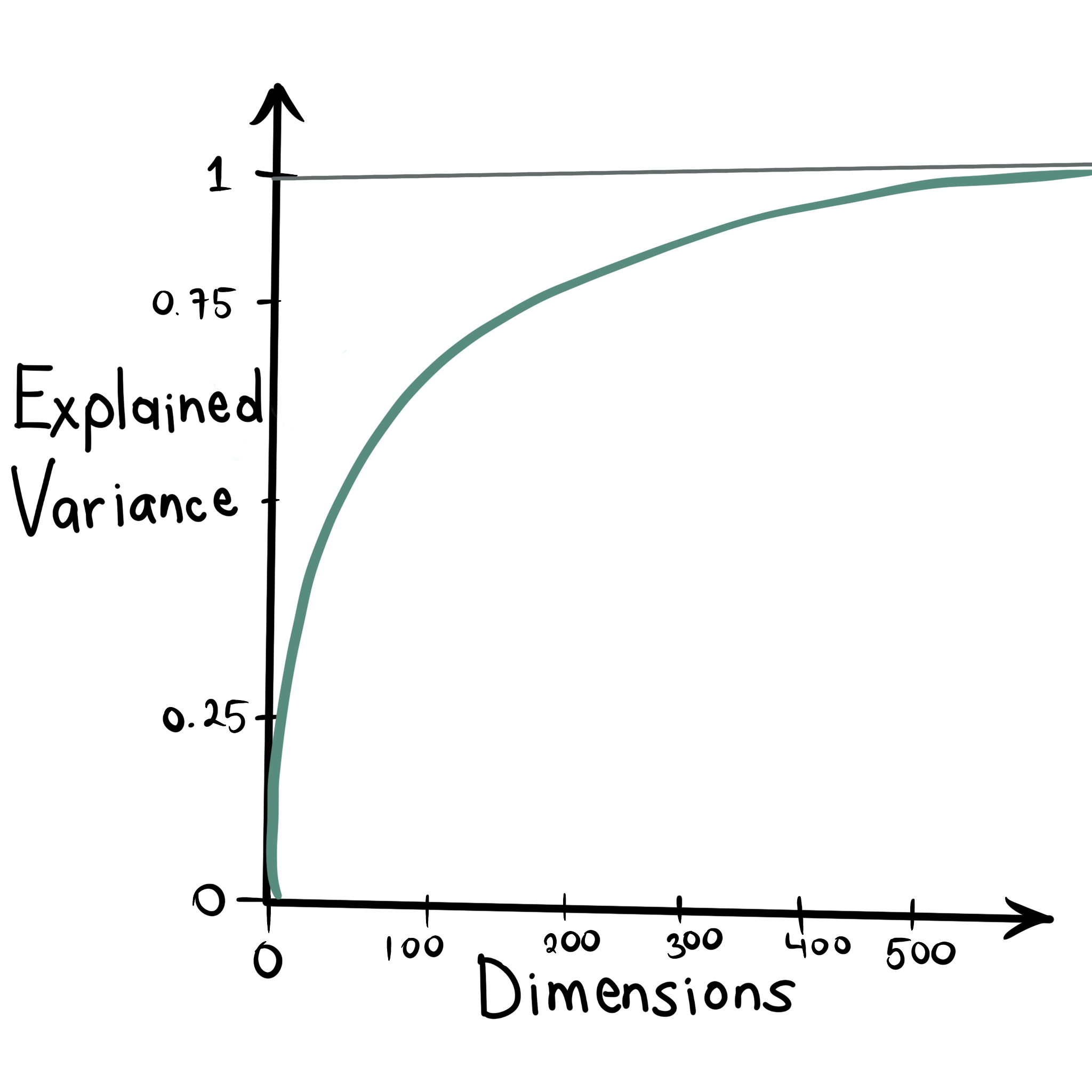
Another way to obtain an optimal number of reduced features is by giving the percentage (or proportion) of information we want to keep.
Classifier: Support Vector Machine
Support Vector Machine (SVM) is one of the most elegant algorithms in Machine Learning, also one of the most powerful. With the correct pre-processed data, the performance of SVM can be at the height of Artificial Neural Networks like in the article Dimensionality Reduction for Handwritten Digit Recognition [3]
One of the particularities of this algorithm is the kernel trick. This technique transforms the dimensions of the data without compromising computational performance so it can be linearly separable [1].
There’s a technique to tackle nonlinear problems that add features computed using a similarity function, which measures how much each instance resembles a particular landmark. The Gaussian _Radial Basis Function_ is a similarity function that, alongside the magic of the kernel trick, leads to incredible results on SVM.
![Figure 4. An example of how the Gaussian RBF transforms the data. The original feature is x1; x2 and x3 are the features created by the Gaussian RBF. Inspiration from [1].](https://miro.medium.com/1*LdnDRgofn9wAfU2EX47knA.png)
Equation 3 shows us the Gaussian RBF kernel, where a and b are hyper-vectors and 𝛄 (gamma) is a hyper-parameter. Increasing 𝛄 makes de bell-shaped curve narrower (increase 𝛄 if the model is underfitting) causing that each instance’s range of influence smaller and, reducing 𝛄 makes the bell-shaped curve wider (reduce 𝛄 if the model is overfitting) causing the opposite effect.
The Pipeline
Besides the processes discussed, previous to the SVM classifier, the data have to be at the same scale; hence the
StandardScaler.Also, a new class had to be made in order to implement HOG in the pipeline
The first model
Metrics
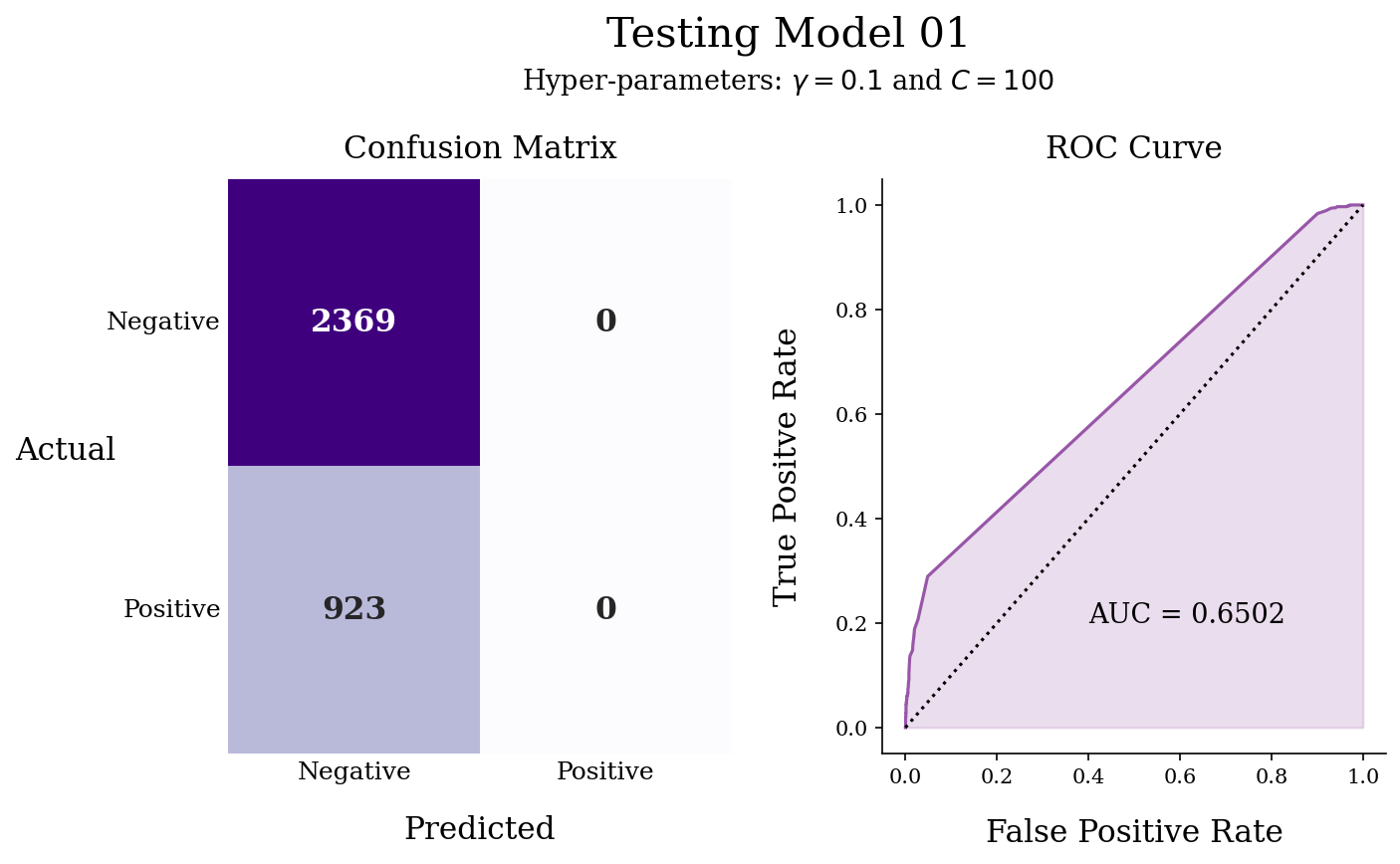
Accuracy: 0.71962 Precision: 0 Recall: 0 F1-Score: 0
Discussion
Low performance is obtained with this model and its hyper-parameters. The confusion matrix shows high True Negatives leading to a high accuracy; however, there is no detection of true positives, resulting in all other metrics with values of 0.
Fine-tuned model
To improve the model’s performance, the hyper-parameters must be modified. Doing this task manually and keeping track of the performances is tedious and tiring; for this GridSearchCV is used.
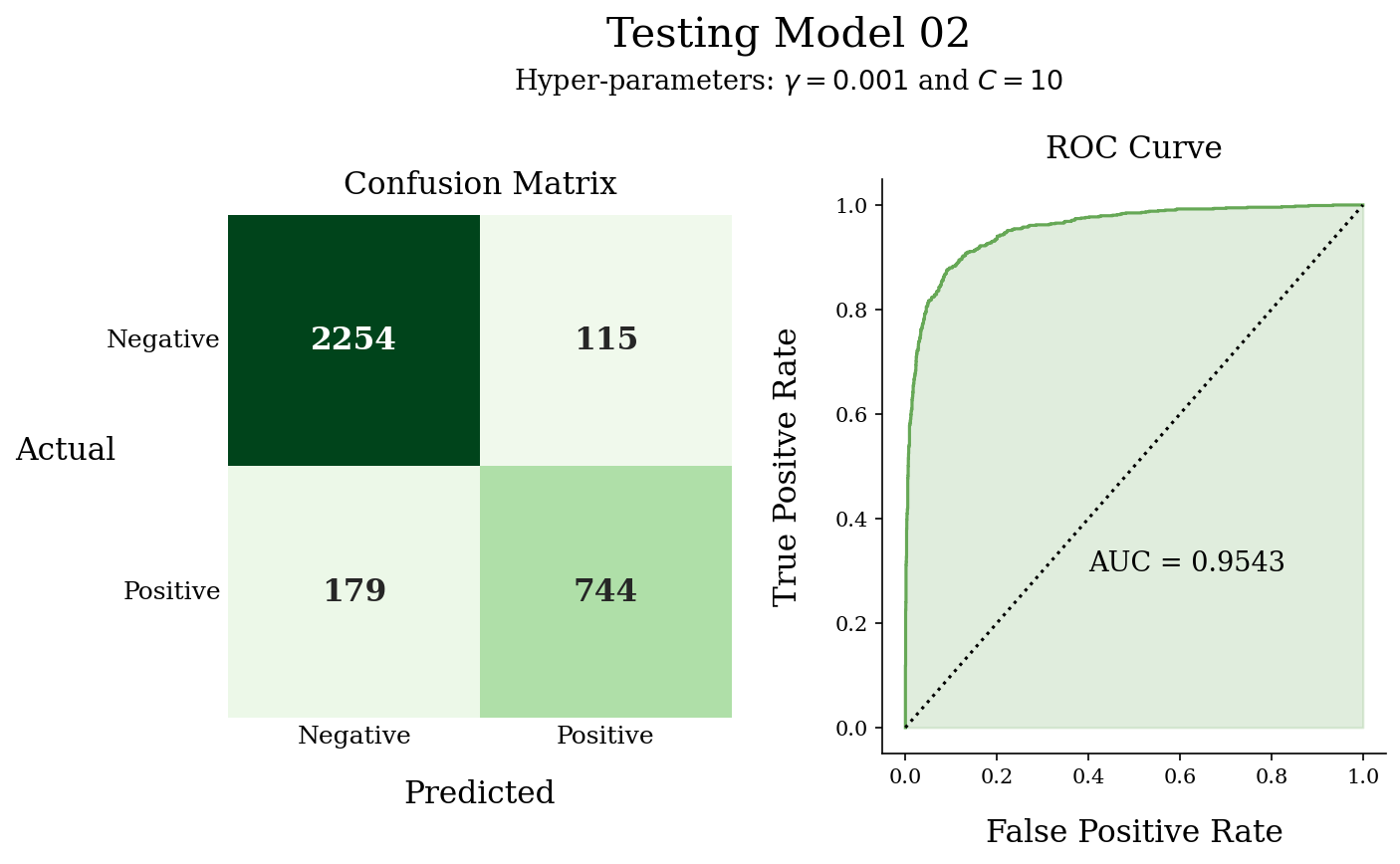
Metrics
Accuracy: 0.91069 Precision: 0.86612 Recall: 0.80606 F1-Score: 0.83502
Discussion
After applying GridSearchCV, the best hyper-parameters for the SVM are found and compared to the previous model; the predictions improve by far. Moreover, the model achieves a high percentage and good balance for classifying positive class faces that are actually correct from those predicted without many false alarms.
The ROC AUC and the shape of the ROC curve show a good prediction model.
Conclusions
About the project
Thanks toGridSearchCV, the model’s best hyper-parameter were found, and in that way, the model achieved high scores in Precision, Recall and consequently F1-Score. It’s important to clarify that GridSearchCVis not about creating a grid of random numbers. Knowing how these hyper-parameters affect the algorithm makes the difference between a good and poor execution.
Support Vector Machine is capable of many things. This project has shown how this algorithm takes abstract features of an n-dimensional space and manages a way to make a reasonable classification.
Future work
The next step of this project is to use the final model in some application or implement it on an external device such as a Raspberry Pi with a webcam.
About what I learned (personal opinion)
During this project, I could explore more about Feature Extraction processes such as HOG and PCA. Although HOG is no longer a state-of-the-art technique, understanding the underlying computations is never a bad idea. The concept is better digested once applied to a project.
Taking complex problems, which have been treated with Deep Learning, and trying to solve them with classical Machine Learning algorithms can help better understand concepts seen and the application of new ones. I also believe that doing this shows the ability to solve problems by taking different perspectives on the same situation.
Repository
GitHub – isaacarroyov/fer_without_ann: Machine Learning Project where the approach to a Facial…
About me
I’m Isaac Arroyo, an Engineering Physicist. I visualize myself solving different kinds of problems by using Data Science and Machine Learning tools. I’m interested in Data Visualization and Unsupervised Learning.
You can contact me or follow up on my work and experiences via social media (Instagram, Twitter or LinkedIn) here. I also create content in English and Spanish.
References
[1] Géron, A. (2019). Hands-On Machine Learning with Scikit-Learn, Keras, and Tensorflow: Concepts, Tools, and Techniques to Build Intelligent Systems (2nd ed.). O’Reilly Media.
[2] Dalal, N., & Triggs, B. (2005, June). Histograms of oriented gradients for human detection. In 2005 IEEE computer society conference on computer vision and pattern recognition (CVPR’05) (Vol. 1, pp. 886–893). Ieee.
[3] Das, A., Kundu, T., & Saravanan, C. (2018). Dimensionality reduction for handwritten digit recognition. EAI Endorsed Transactions on Cloud Systems, 4(13).


